Route types and how they're optimized differently

Each delivery run has its own flavour depending on the purpose of the run. A very simple fixed delivery run varies significantly to a daily dynamic pick up and drop off run with multiple stops at a depot. The truck type, terrain, schedule, cargo, and stop structure all introduce variations that mean each route needs to be optimized on an individual basis – there is no one size fits all optimization. 

Delivery route types

Before we look at how to optimize routes, let’s see how they can be categorized: 

By stop structure

Milk run
A milk run is a fixed, recurring route visiting the same stops in the same sequence, typically on a set schedule. This run type is common in manufacturing supply chains and regular replenishment runs.

Point-to-point (P2P)
A run from a single origin to a single destination, common in same-day courier and urgent freight logistics.

Multi-drop
Starts from one origin with multiple delivery stops and no pickups, basically the classic "delivery run."

Pickup and drop-off (PUDO)
PUDO mixes collections and deliveries on the same route. It is significantly more complex to optimize due to load sequencing constraints, however a dynamic route can respond to changes in conditions (such as a missed delivery) and incorporate an extra stop in an ad hoc way that gains an optimization during the re-delivery.

Hub-and-spoke last mile
Named after the design of a wheel, cargo is consolidated at a depot or micro-fulfilment centre (the hub) before being distributed outward on radial routes (the spokes.)

Cross-dock run
Cargo is transferred between vehicles at a transfer point without storage. It is often time-critical and sequencing-sensitive.

By scheduling type

Fixed/set runs
A pre-planned route with locked stops and sequence. This is a stable route but can become inefficient over time if not reviewed. See an example: StarTrack Courier found runs unchanged for 10 years before re-evaluating them with Adiona.

Dynamic or on-demand route
Stops are added to a route in real time as orders come in. With this method, volumes can fluctuate dramatically especially during peak time. Being able to respond to this fluctuation  with dynamic route optimization becomes your superpower.

Pre-planned with ad-hoc additions
A hybrid of dynamic and a milk run, where a base route is planned in advance but exceptions and urgent stops are inserted throughout the day.

By cargo and service level

Time-window delivery
Multiple factors can introduce strict delivery time windows, such as a perishable cargo or busy loading dock that needs to efficiently receive orders from multiple trucks. This is extremely common in B2B restocking (for example: retail, pharmacy, FMCG.)

Appointment-based delivery
Common for bulky freight and healthcare, the recipient agrees on a specific delivery time, with high consequences if the delivery is missed. 

Same-day delivery
Orders are placed and delivered within the same day, requiring dynamic routing and tight ETA accuracy.

Time-critical and emergency runs
Delivering life-critical cargo such as blood, organs, or medical equipment with zero tolerance for latency or re-routing requires dedicated algorithms that prioritise time over cost.

Temperature-controlled runs
Refrigerated or frozen cargo often has dwell-time constraints at each stop. Route sequencing should account for how long or how frequently doors are opened and the extra energy consumption of the vehicle.

Hazmat or restricted cargo runsRoutes for dangerous goods may be constrained by road classifications, tunnel restrictions, or permit zones.

By fleet and vehicle type

Full truckload (FTL) last mile
Routes are serviced by large vehicles completing a single delivery or very few stops, typically to a DC or large retail customer.

Less-than-truckload (LTL) consolidation runs
Multiple consignments from different shippers are consolidated onto one vehicle.

Parcel or courier runs
These runs have a high stop count with a low dwell time per stop. Optimization is heavily focused on sequencing and territory clustering.

Bulky goods runs
These runs have a lower stop count, longer dwell time, often requiring two-person crews to move cargo in and out of the vehicle. Vehicle load sequencing (last-in-first-out) is critical and adds an extra dimension to route planning.

EV-optimized runs
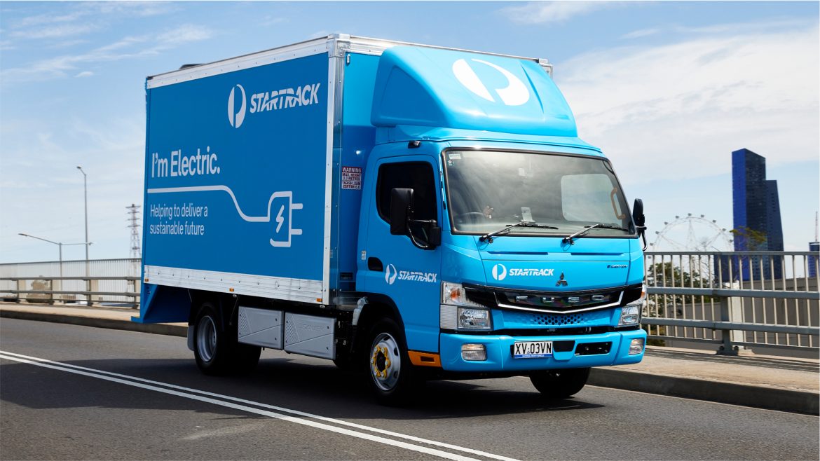
Routes are designed around battery range, charging infrastructure, payload weight, altitude, and ambient temperature, among other EV-specific factors. Adiona's EV fleet simulator accounts for all of these variables.

By territory structure

Zone-based and territory runs
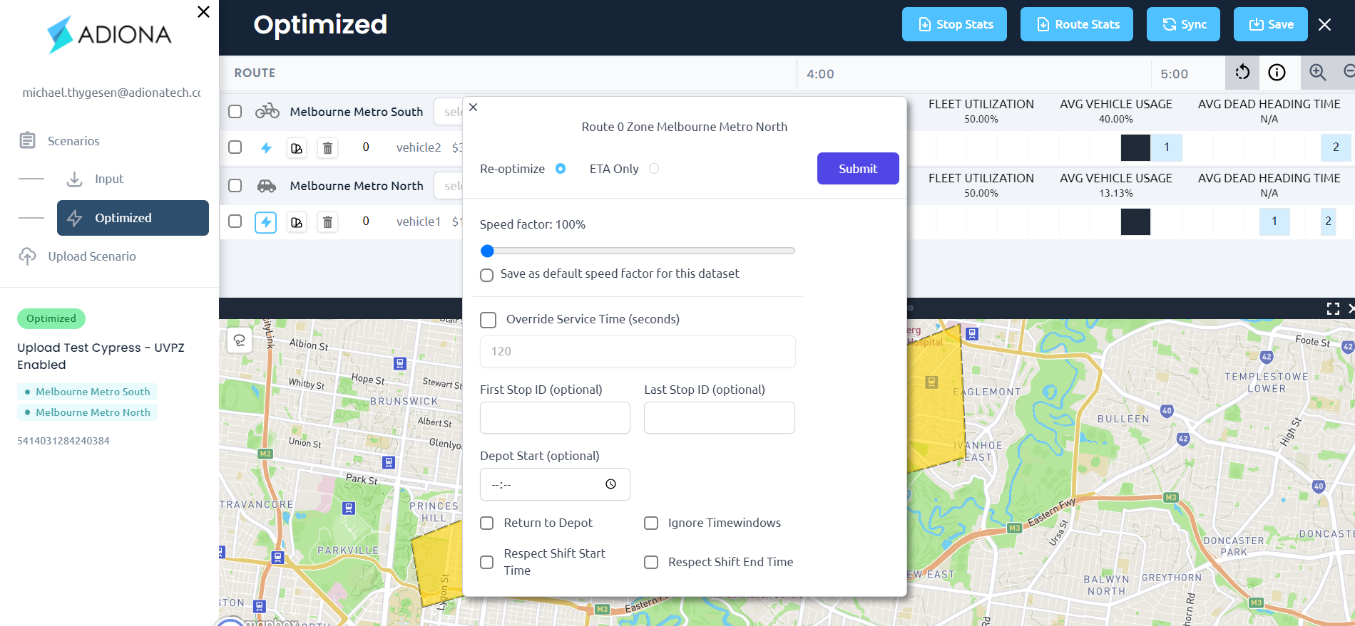
Each driver is assigned a geographic zone and owns all deliveries within it, creating consistency but can also create inefficiencies at zone boundaries or become out of date as soon as a new customer is added. Read a case study about territory balancing with Adiona.

Interleaved or pooled territory
Stops are assigned dynamically across zones to maximise vehicle utilisation, especially during volume spikes.

Radial run
Routes emanate from a central point (depot) outward, typically structured to minimise backtracking. This sounds similar to the hub and spoke model above, the distinction is a hub and spoke approach is for the network itself, while a radial run is a single run within a network. A hub and spoke network often has radial runs within it. 

Loop run
‍The route forms a closed circuit returning to the depot, optimized for total distance rather than individual stop sequence.

Corridor run
A linear route follows a geographic corridor (e.g. a highway strip or main arterial), common in regional or long and thin geographies or territories.

By driver or operational model

Owner-driver run
Where a fleet uses independent contractors with a fixed territory the route optimization must respect contractor agreements and earnings expectations.

Crowdsourced or gig delivery
Routes are assigned dynamically to casual drivers, with a heavy reliance on real-time optimization.

Multi-shift runs
The same route or territory is covered across two or more driver shifts, requiring handover planning and depot return sequencing.

Driver redeployment run
After completing a primary run early, a driver is reassigned to a secondary run. Requires real-time optimization capability to identify and assign the next best task.

By network complexity

Single depot, single shift
The simplest configuration and the most common starting point for optimization.

Multi-depot
Routes can originate from or return to different depots, with the optimizer selecting the best depot per route or stop.

Micro-fulfilment centre (MFC) routes
Last-mile routes originate from a small urban fulfillment node rather than a traditional depot, enabling faster same-day coverage in dense urban areas.

Relay or linehaul with last mile
Long-haul leg transfers to a local delivery vehicle at a transfer point and the last-mile leg is then optimized separately.

How each delivery route type is optimized

Given we now understand just how unique each route type is, it’s safe to say that optimizing each type requires its own approach. In many cases, logistics businesses mix route types, network types, driver types, and vehicle types in one big, complicated mix. 

Many routing tools can’t handle this complexity and apply a one-size-fits-all approach, forcing route planners to manually optimize and constantly tweak routes until they’re ‘good enough’. 

Let’s take a look at the factors that get considered in each route type when optimizing the runs.

Pickup and Drop-Off (PUDO) Routes

Unlike a pure delivery run where every stop is a drop, PUDO routes require a vehicle to collect items from some locations and deliver them to others, often within the same shift and sometimes within tight time windows.

The challenge is created by the fluctuation in the vehicle’s capacity; A driver can't deliver something they haven't yet picked up, which means the optimization engine has to respect a web of precedence constraints — stop B must come after stop A, stop D after stop C and so on.

This gets particularly complicated when you have multiple pickup-delivery pairs interleaved across the same route. A naive routing engine will struggle here, defaulting to geographically close clusters that inadvertently violate the pickup-before-delivery ordering. A good optimization engine handles PUDO with a dedicated algorithm built specifically for this constraint.

StarTrack Courier — Australia Post's same-day courier arm — is a strong example of a PUDO-heavy operation. Their fleet handles everything from e-commerce returns to medical specimens, all with tight sequencing requirements. When they evaluated route optimization platforms, a robust PUDO algorithm was a non-negotiable requirement. It was one of the reasons they selected Adiona, which has a dedicated PUDO algorithm built into the platform. You can read more about their implementation in the StarTrack Courier case study.

Milk runs

Milk runs are often seen as "set and forget" from a planning perspective. The route was optimized once, years ago, and has been running on autopilot ever since. This is exactly the thinking that quietly erodes fleet efficiency over time.

Once customer volumes change or traffic patterns shift a milk run that was once tightly optimized can develop significant inefficiencies such as wasted distance, unnecessary stops, or poorly timed arrivals.

The opportunity in milk run optimization is in ongoing route reviews. Routing teams at StarTrack Courier discovered exactly this when they started running existing routes through Adiona's platform. As Christopher Cano, their National Business Improvement and Implementation Manager, put it: "The guys are looking at their runs and saying they haven't changed in 10 years, now we have Adiona so let's run it through there." The results consistently revealed savings that had been invisible under the old approach. Read more in our case study on optimizing existing runs with StarTrack Courier.

For milk run optimization, the key inputs are historical volume data, realistic dwell times at each stop, and current traffic patterns.

High-density metropolitan runs vs. low-density suburban and rural runs

These two route types require fundamentally different optimization strategies:

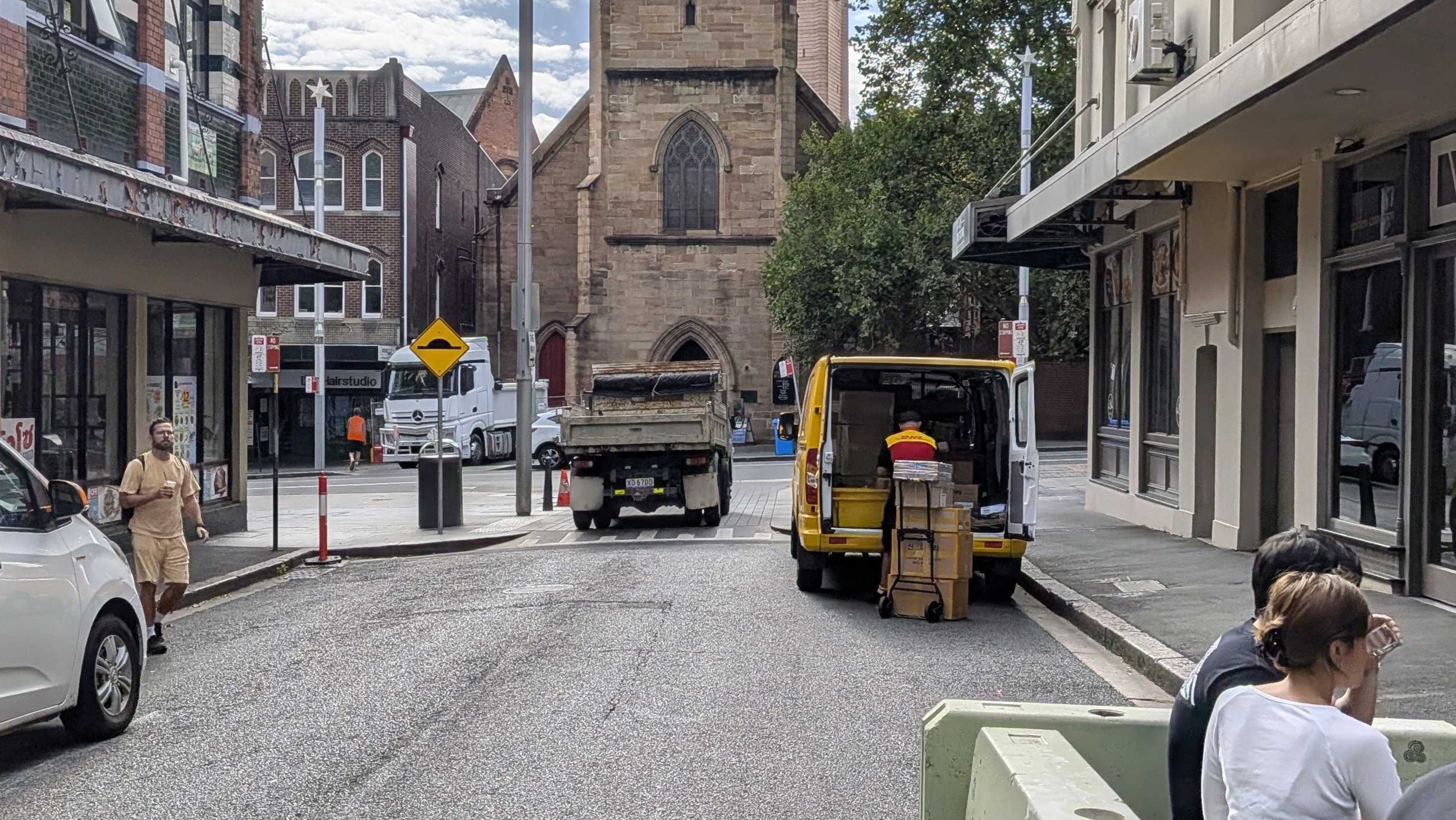
High-density metropolitan routes are dominated by dwell time and traffic, not distance. When stops are close together (for example, inner-city deliveries to office towers where addresses are 50 to 200 metres apart) the time between stops is negligible. What matters is how long the driver spends at each stop to find parking, navigate a building lobby, deal with access codes, or manage failed delivery attempts. In a dense urban environment, route optimization has to account for traffic congestion by time of day, parking availability and restrictions, building access constraints, and the sequencing of stops within a single block or precinct to minimise backtracking on foot.

Low-density suburban and rural routes flip this equation. Here, drive time between stops dominates the shift, and the cost of a suboptimal sequence is measured in kilometres and litres of fuel rather than minutes of parking. The optimization challenge shifts to minimizing total distance while respecting time windows and managing the vehicle's capacity across a longer day. These routes are also more sensitive to road type. A straight-line distance between two rural stops can translate into a much longer actual drive if the road network requires detours.

The practical implication for fleet managers is that a single optimization approach doesn't work well across both contexts. Operations running both urban and suburban routes benefit from software that can handle different constraint profiles for different route types within the same platform.

Maintenance and service vehicle runs

Maintenance vehicles often return to depot multiple times throughout a day to collect parts, drop off recovered equipment, or re-stock before the next job.

This creates a multi-leg routing problem. Each "trip" from the depot is effectively a mini-route, and the sequencing of jobs across trips has to account for parts availability, job duration uncertainty, and the cost of each return journey. A vehicle that makes four depot returns in a day needs four optimized outbound legs, not one.

Technician skill sets add another layer of complexity. Not every technician can complete every job, so routing has to respect job-to-technician matching alongside geography and timing. Priority escalations such as an emergency repair that lands mid-morning can force real-time re-sequencing of the entire day's remaining work.

Fleet management teams operating service vehicles benefit enormously from optimization tools that handle multi-trip routing natively, rather than planning each depot departure as a separate route with no awareness of the others.

Electric vehicle routes

EV fleet routing is a category that is growing rapidly, and it introduces constraints that conventional routing engines weren't designed to handle.

Range anxiety has largely been alleviated by the early fleets who have trialled and proven an EV can complete runs without running out of battery. However, the battery does introduce a range of factors that can be used in the route optimization: cargo weight, climate, altitude changes, driving speed, acceleration, inclines, and whether the heating or air conditioning is running.

For fleets transitioning from ICE vehicles to EVs, there's an additional planning challenge: which routes are suitable for which EV models? A 150km suburban route might be straightforward for one EV but marginal for another depending on its battery capacity and the route's elevation profile. Running these scenarios against real data before committing to a vehicle purchase is where simulation tools become invaluable.

Adiona's FlexOps Fleet Simulator allows fleet operators to model different EV types against their actual route data and account for battery performance, range, cargo weight, temperature, and more before making purchasing decisions. The platform also integrates emissions tracking at the parcel level, supporting organizations working toward Net Zero targets. You can explore this capability in detail on the Adiona EV fleet optimization page.

Refrigerated and temperature-controlled routes

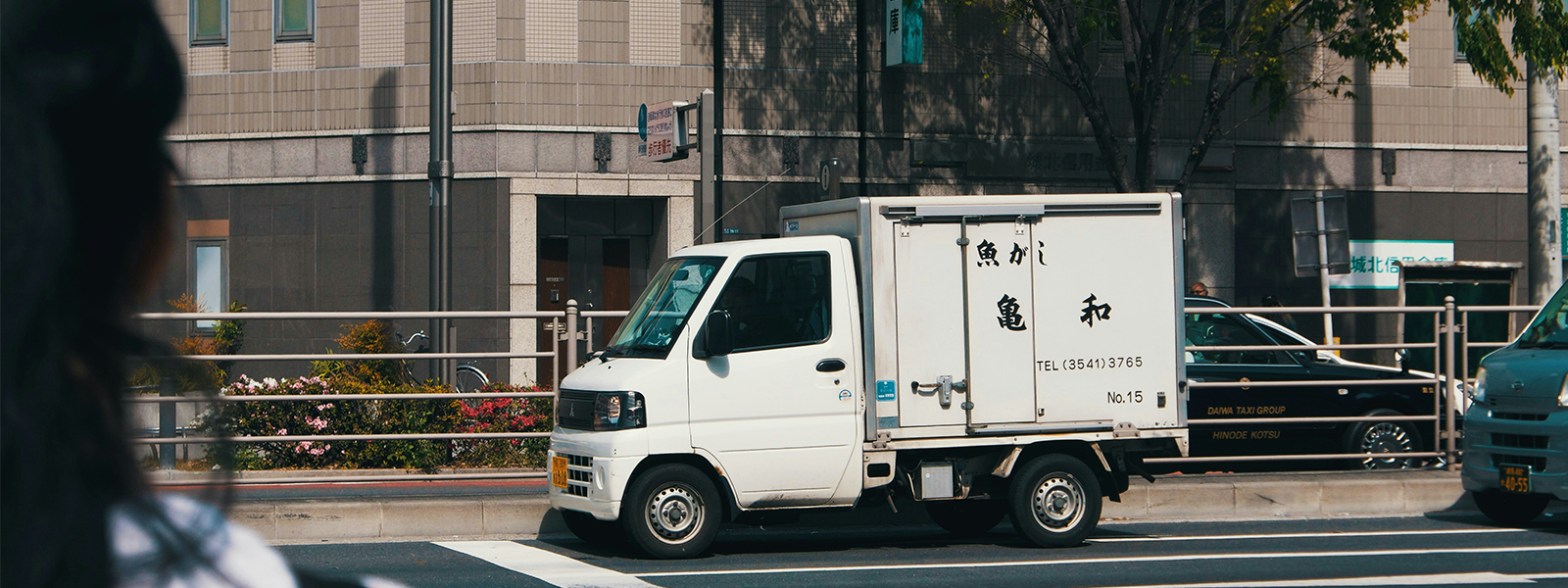
Cold chain delivery adds another factor to account for – keeping the cargo the right temperature. At first this sounds simple, but something as obvious as opening the truck up to load or unload cargo can mean serious temperature fluctuations and the truck working harder to continuously bring the hold back to the right temp. 

The optimization implication is that it's not just about the most efficient sequence of stops. It's about the sequence that minimizes how many times the truck needs to be opened up. If two stops are close together and the driver can park once, unload both deliveries, and deliver the second stop on foot rather than driving, parking, and unloading a second time, the fuel savings will add up.

Some cold chain operations run mixed loads (ambient and chilled product in partitioned compartments) which adds further constraints around which compartment doors are being opened at each stop. Time windows are also typically tighter for cold chain customers, particularly in food service and pharmaceutical delivery, where products must arrive within a strict temperature band.

For routing teams managing refrigerated fleets, the combination of time windows, stop clustering for thermal efficiency, and load sequencing makes this one of the more complex optimization problems in last-mile delivery.

Third-party logistics fleets vs. dedicated fleets

The operational dynamics of a 3PL fleet and a dedicated fleet are quite different, and this flows through into how routing should be approached for each.

A dedicated fleet operates for a single customer or a single brand. Routes are planned around that customer's network, service level agreements, and delivery commitments. The planning team has full visibility of the cargo, the customer base, and the service standards. Optimization is a matter of finding the best sequence given a known, bounded problem.

A 3PL fleet carries multiple customers' freight simultaneously. This introduces complexity at almost every level. Different customers have different service level requirements, different packaging specifications, different delivery time windows, and different relationships with the end recipients. Some customers may have exclusivity requirements and don't want their freight on the same vehicle as a competitor's product. Others may have specific handling instructions that affect how the vehicle is loaded and in what order stops can be made.

For 3PL operators, route optimization also has a commercial dimension. Being able to demonstrate to prospective customers that their freight will be handled efficiently is increasingly a differentiator in winning contracts. This is exactly the use case that StarTrack Courier's team found when they started using Adiona's route simulation capability to model service levels for new business proposals. As Christopher Cano noted, the ability to present "professional looking outputs from Adiona" rather than patchy Excel spreadsheets transformed the quality of their commercial conversations. Read the full story in our case study on winning new business with route optimization.

Hub-and-spoke networks

Hub-and-spoke is a network design model rather than a single route type, but it has significant implications for last-mile route planning. In a hub-and-spoke model, freight moves from origins to a central hub before being redistributed to final destinations via spoke routes.

For last-mile operators, the relevant challenge is at the spoke end. How do you design and optimize the delivery routes that radiate out from each hub to serve the surrounding catchment? The answer depends heavily on the density of demand in each catchment, the vehicle types assigned to each spoke, and the service level commitments for each delivery territory.

Hub-and-spoke networks also raise questions about depot sizing and placement. Where should a new hub be located to minimize the total distance travelled across all its spoke routes? How many vehicles does each hub need to service its territory within the required time windows? These are depot and network planning questions that sit above individual route optimization but have a direct bearing on it.

Adiona's FlexOps platform includes depot simulation capabilities that allow operators to model different hub configurations against real demand data before committing to infrastructure changes, a particularly valuable tool when evaluating micro-fulfilment strategies or planning network expansions.

Return to depot vs. finish at home

The question of where a driver's day ends is more consequential for route optimization than it might first appear.

In a return-to-depot model, the driver finishes their shift back at the starting location. The optimization problem is a closed loop where the route begins and ends at the same point, and the planner is looking for the most efficient circuit. This model is common in bulk delivery, field service, and operations where vehicles need to be inspected, loaded, or maintained overnight at a central facility.

In a finish-at-home model, the driver finishes their last delivery and goes directly home, and the vehicle may stay at their residential address overnight. This is common in courier and parcel operations where drivers are assigned a territory close to where they live, and it opens up genuinely different optimization possibilities. The planner can optimize for an open-ended route that ends wherever makes geographic sense rather than looping back to a depot.

The finish-at-home model typically produces shorter total routes, since drivers don't need to drive back across the city at the end of a long shift. But it introduces fleet management considerations around vehicle security, overnight parking, and the morning start. If vehicles are dispersed across a metropolitan area, how does each driver get to their vehicle at the start of the day?

Daily dynamic routing vs. fixed routing

This is perhaps the most fundamental choice in route planning strategy, and the right answer depends heavily on the nature of the demand.

Fixed routing assigns specific customers to specific routes and drivers on a predictable schedule. The routes are planned once and repeated, with only minor adjustments as needed. Fixed routing is appropriate when demand is stable and predictable, when drivers benefit from building relationships with regular customers, when customers expect the same driver at the same time each visit, or when loading and dispatch processes are built around a consistent sequence.

Dynamic routing generates route plans every day (or each shift) based on that day's actual orders. No two days look the same. Dynamic routing is appropriate for operations where order volumes fluctuate significantly day to day, the geographic spread of demand changes, or where same-day and next-day delivery commitments require routing against real-time order data.

Many operations sit somewhere between these poles: a fixed backbone of regular customers with dynamic capacity for ad-hoc orders layered on top. Managing this hybrid effectively requires tooling that can hold fixed route commitments while dynamically filling available capacity, a more nuanced problem than either pure fixed or pure dynamic routing alone.

StarTrack Courier's same-day operation is a good example of dynamic routing in practice. As Christopher Cano explained, daily volumes can fluctuate by as much as 40% across the month. Adiona's platform allows his team to input the day's manifest and quickly generate viable route plans that account for actual driver availability, a process that was previously manual, slow, and dependent on institutional knowledge. See how this works in practice in the day-to-day routing case study.

Parcel delivery routes

High-volume parcel delivery is one of the most studied last-mile problems in logistics, and for good reason, it's also one of the most economically significant. At scale, marginal gains in parcel route optimization compound dramatically.

The defining characteristic of parcel routes is volume. A typical parcel driver might have 80 to 150 stops in a shift, often across a dense residential area. At this scale, the sequencing of stops within a street, the choice between clockwise and anticlockwise traversal of a loop road, and the timing relative to traffic peaks all have a measurable impact on the number of deliveries completed per shift.

Capacity utilisation matters here too. A well-optimized sequence that leaves the vehicle over-loaded at the start of a run is useless if the driver can't physically access the parcels for early stops because later stops are blocking them. Load sequencing (planning the physical loading of the vehicle in reverse delivery order) is a non-trivial part of the optimization for parcel operations.

Failed deliveries add another dimension. When a parcel can't be delivered, the rerouting decision (attempt again today, return to depot, redirect to a collection point) affects the rest of the day's route. Dynamic routing platforms handle this more gracefully than static plans, which tend to treat failed deliveries as an afterthought.

Adiona's FlexOps platform consistently increases delivery capacity for parcel operations. One client reported moving from 7 deliveries per truck to 10 or 11, a change that became, as their National Warehouse and Logistics Manager Talal Kanj put it, "automatic with Adiona's platform."

One side of the road at a time

For route types like waste collection, the routing has a constraint where it needs to complete the entirety of one side of a street at a time. Crossing the road, and the traffic, repeatedly to service both sides is unsafe and operationally impractical with large refuse vehicles.

This means a typical residential street requires two passes, one for each side. So how do you plan the order of streets and the direction of travel through each one so that both sides of every street are covered while minimising total distance and avoiding the vehicle having to double back unnecessarily?

This is a variant of the classic "Route Inspection Problem" in route planning. It’s not finding the shortest path through a set of points, but finding the most efficient traversal of a set of edges. Conventional point-to-point routing algorithms aren't designed for this, which is why waste collection routing is often handled by specialist software or, in smaller operations, by experienced planners who know their territory intimately.

The one-side constraint also interacts with vehicle size. A large refuse vehicle turning around at the end of a dead-end street has very different handling requirements to a courier van, and the route plan needs to account for whether turnarounds are physically possible at each point.

Big and bulky deliveries with multi-person crews

Furniture, white goods, large appliances, and other oversized items introduce crew-level constraints that standard parcel routing ignores entirely.

The first is simply time. A two-person crew delivering and installing a washing machine might spend 20 to 40 minutes at a single stop. At this dwell time per stop, a bulky goods run might have 8 to 15 stops in a full day's shift rather than the 80 to 150 of a parcel route. Every minute of drive time matters proportionally more.

The second is access. Large items require vehicle access close to the delivery point, which means planning routes that avoid stops where a large van or truck can't get close to the door. Apartment deliveries require lift access (or carrying up stairs) and advance confirmation of building access. Customers who won't be home are particularly costly — a failed bulky goods delivery often can't be re-attempted the same day, and the item has to go back to the depot.

Third is crew scheduling. Multi-person delivery teams have their own rostering constraints, and the route plan needs to keep the crew together throughout the day. 

For fleet managers running bulky goods operations, accurate dwell time data at the stop level is the single most valuable input to the optimization. An optimization model that assumes 5-minute stops for furniture delivery will generate plans that are impossible to execute.

Micro-fulfilment vs. large depot runs

Where freight starts its last-mile journey has a significant bearing on how the route should be planned.

Large depot runs originate from a regional distribution centre, typically on the outskirts of a metropolitan area where land costs are lower and freight volumes justify the infrastructure. Drivers load their vehicles at the depot, then travel (often some distance) to their delivery territory before beginning their stops. The return journey at the end of shift is the reverse. The optimization question is how to assign delivery territories to drivers so that each driver's total time is balanced and efficient.

Micro-fulfilment relocates inventory much closer to the point of demand, often into small urban facilities, dark stores, or shared retail back-of-house spaces. The goal is to reduce the distance between stock and customer, enabling same-day and rapid delivery at lower per-delivery cost. Routes originating from a micro-fulfilment location are typically shorter and more densely packed than those from a regional depot, because drivers start their routes much closer to where their stops are.

The trade-off is inventory management complexity. Smaller fulfilment nodes hold less stock, which means more frequent replenishment runs and a higher risk of stockouts for fast-moving lines. Micro fulfillment centres also have replenishment runs to route for, adding more work to a planner’s day.

Adiona's FlexOps platform includes depot simulation capabilities, allowing operators to model different fulfillment configurations against real demand data before making infrastructure commitments.

Real constraints require real optimization

Reading through these route types, a pattern emerges. Every single one of them has constraints that a generic routing approach handles poorly: precedence constraints in PUDO, thermal constraints in cold chain, range constraints in EV routing, side-of-road constraints in waste collection, crew constraints in bulky goods.

Good last-mile optimization isn't about applying a single algorithm to every problem. It's about having an optimization platform flexible enough to model the specific constraints of each route type, and smart enough to find genuine improvements within those constraints rather than defaulting to solutions that look good on paper but fall apart when the driver hits the road.

This is also why the "set and forget" approach to route planning is so costly. Routes that were optimized five or ten years ago, under different demand patterns and different network configurations, rarely reflect the best possible plan today. The operations teams that get the most from route optimization are those that treat it as a continuous process, regularly revisiting existing runs, testing new configurations, and using data to challenge assumptions that have calcified into habits.

If you're managing a fleet and wondering whether your current routes are really optimized or just familiar, the honest answer is almost certainly that there's room to improve. 

Ready to explore Adiona?

Whether you're running PUDO routes, managing a cold chain operation, planning an EV transition, or trying to win new contracts with credible route modelling, the starting point is the same. Put your actual operational data into Adiona free for 14 days and test the optimizations for yourself!

Explore the FlexOps platform or get in touch with the Adiona team to discuss what optimization could look like for your specific operation.